Politics Is Context, Not a Trading Signal

Political averages are irresistible.

They offer a clean sentence after an election, a colorful chart in a client deck, and the pleasing illusion that history has already cast a vote on the next four years.

They are also very easy to overread.

I rebuilt a familiar claim—that one political configuration is better for U.S. equities than another—using only the frozen public data captured for this project. The result is not that politics are irrelevant. Tax policy, regulation, fiscal choices, trade, and industrial policy plainly matter for companies and sectors.

The result is narrower and, I think, more useful:

Political labels are useful for framing scenarios. They are poor standalone inputs to a broad equity-allocation rule.

The public reconstruction finds a descriptive ranking of historical returns by party and congressional control. But the leading cell has only eight annual windows across three administrations; 24 of the 87 annual windows change political configuration after their label is set. Meanwhile, a basic starting valuation measure shows a more consistent descriptive relationship with the following year’s return than the starting policy-rate level does.

That is not a prediction. It is a reminder to start with the opportunity set the market has already priced, rather than treating a party label as a factor that arrived with magical explanatory powers.

The short version

The charts and analysis below come from PRES, the local Presidential Impact workspace I built in QuantMeridian. It loads the project’s frozen public inputs, keeps the comparison definition alongside the figure, and labels the result USER-SUPPLIED · UNVERIFIED: an honest statement that the module validated the data contract and calculations, not a claim that software independently authenticated every historical observation.

• The party-and-control ranking is descriptive, but its leading cell is small and its return windows are not independent experiments.
• The dated control timeline exposes why an annual label is not the same thing as a full-year political treatment.
• Starting CAPE has a clearer negative association with the following year’s return than the starting policy-rate level in this frozen sample.
• None of those observations is a forecast, an allocation rule, or proof that a president caused a return.

The claim I wanted to test

The starting point was Fiduciary Trust International’s October 2024 article, “Should the balance of power in Washington matter to investors?”. It presents a long-run S&P 500 comparison by political configuration and makes the sensible observation that starting fundamentals deserve attention.

The article is a useful research lead, not a dataset I could reproduce exactly. Its annual return analysis cites BofA Global Research, Bloomberg, and FactSet. Those vendor inputs, the underlying calculation table, and several assignment rules are not available here. Relabeling a public approximation as an exact S&P 500 replication would be the sort of confidence trick that makes backtests look great right up until someone asks for the inputs.

So I did not do that.

Instead, I built a clearly labeled public-data reconstruction over the common 1936–2022 annual sample:

• A public CRSP-market-proxy baseline, compounded from Kenneth French Mkt-RF + RF. It is not the S&P 500.
• A separately constructed Shiller S&P Composite dividend-reinvestment-style robustness series, based on Robert Shiller’s public workbook. It is also not an official S&P 500 total-return index.
• A manually reviewed political-control record, with dated House, Senate, and presidential intervals rather than a casual assumption that a January label remains the full-year exposure.

The two market constructions are not interchangeable, but they are a useful discipline against narrating whichever series best flatters a preferred result. Their annual returns have a 0.980 correlation over the shared sample, and their mean annual returns differ by only -0.12 percentage points.

Shared 1936–2022 reconstruction	Result
Annual return windows	87
CRSP-market-proxy mean	12.15%
Shiller reconstruction mean	12.03%
Annual-return correlation	0.980
Windows with a later political-control change	24 / 87

This does not make either series the “right” answer. It says that the broad descriptive ranking does not disappear when the public return construction is changed.

The ranking is history, not a political premium

Under both constructions, the six political-configuration averages preserve the same ordering. That is a modest robustness check on a historical ranking. It is not a causal estimate, because the cells are small, administrations repeat across rows, and the country was not randomized into political regimes.

The category with the highest observed mean—Republican president and Republican Congress—contains eight annual observations across three administrations. Its public CRSP-market-proxy mean is 17.55%; the Shiller reconstruction mean is 18.48%.

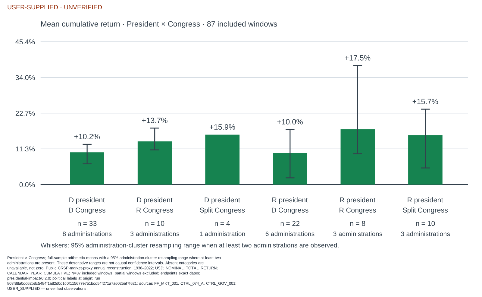
Figure 1. QuantMeridian PRES export using the locked 1936–2022 CRSP-market- proxy common sample. The green bars are arithmetic means; whiskers are 95% administration-cluster resampling ranges, not causal confidence intervals. Every cell is marked with both its annual-window count and its administration count. The orange provenance banner is intentional: these are frozen project-supplied inputs, not vendor-verified market history.

Those numbers may be interesting. They are nowhere near enough to say, “this is the political regime investors should own.” A handful of macroeconomic episodes, valuation starting points, recessions, wars, technology cycles, and market recoveries can do a lot of work inside eight annual rows.

The more important audit is timing. The main analysis assigns political control at the annual window’s start, before the return is known. That avoids a look-ahead label, but it does not turn the whole year into stable political exposure: 24 of 87 windows cross at least one later control change.

In other words, the label is a clean filing system. It is not a clean causal treatment.

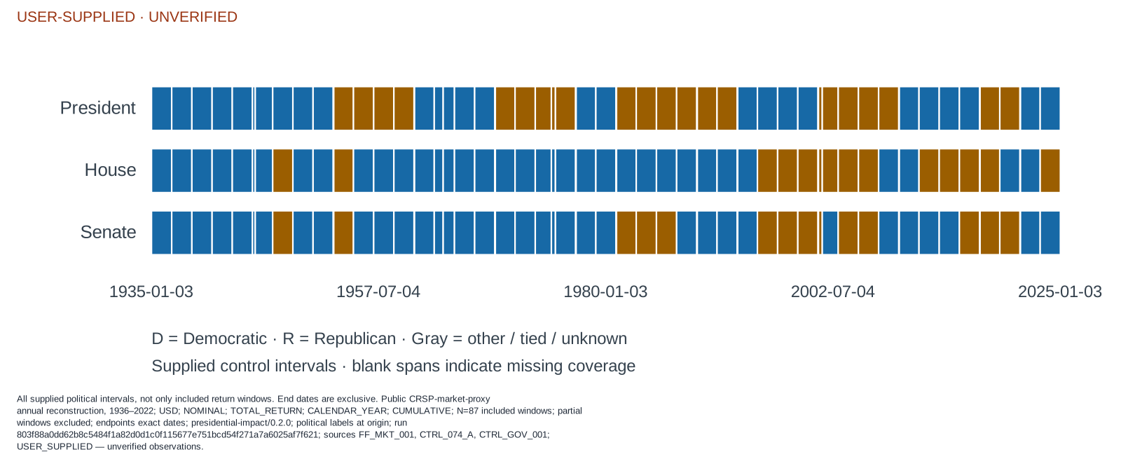
Figure 2. The control timeline behind the annual labels. It uses dated, end-exclusive intervals and includes every supplied interval, not merely the 87 common-sample return observations. This is why a political label at a window’s origin is a reproducible convention—not evidence that control was unchanged for the entire return year.

A presidential cycle has a calendar problem

Presidential-cycle charts are another place where a tidy story can conceal a messy interval. If a calendar year’s return is assigned to the president in office on December 31, the first 20 days of an inauguration year preceded the new regular term’s January 20 start.

That does not make a four-year cycle analysis impossible. It means the transition should be visible.

The chart below summarizes the 86 annual return windows from 1937–2022 under an end-of-calendar-year presidential assignment. The vertical range is the historical minimum to maximum in each party/cycle cell; the diamond is the arithmetic mean. These are observed dispersions, not confidence intervals.

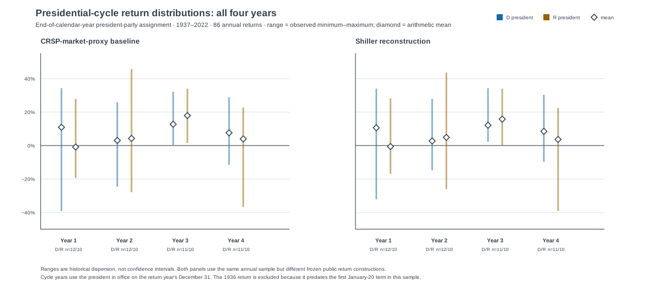
Figure 3. All four cycle years, using the president in office on each return year’s December 31. The 1936 return is excluded because it predates the first January-20 presidential term in this sample. D/R colors identify the end-of-year president’s party; they do not identify a causal exposure.

The companion view keeps every number exactly the same and flags the 22 cycle-year-1 observations as inauguration transitions. Twelve of those 22 windows also have a different president at the annual start and end. The other ten still deserve the timing flag: a re-elected president may be the same person, but a new regular term still begins on January 20.

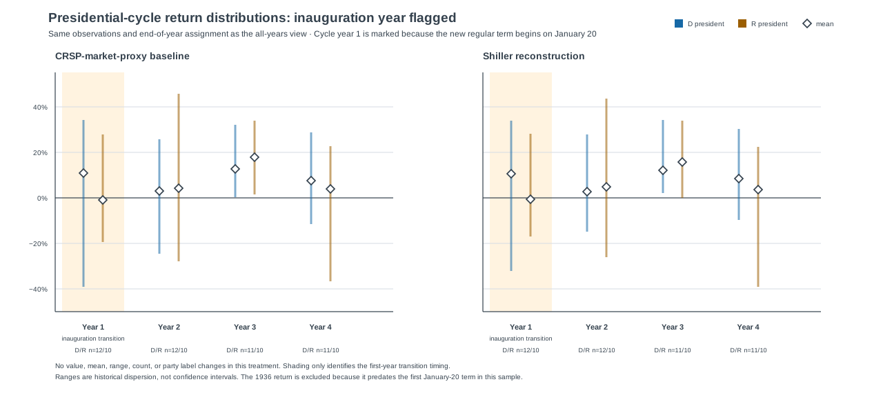
Figure 4. The inauguration-year treatment changes no return, count, party label, range, or mean. It only makes the calendar boundary visible.

The point is not that an inauguration year should be thrown out, relabeled, or used to invent a better political result. The point is to resist giving an end-of-year label more causal credit than the calendar can support.

Starting valuation produced the stronger descriptive pattern

The more interesting question is not “which party won the historical table?” It is “what did the market look like before the return occurred?”

For the frozen 1955–2022 extension, I aligned each annual outcome with the previous October’s Shiller CAPE field and effective federal funds rate, using a one-month assumed-availability lag. The alignment gives 68 annual return windows, tested against both public return constructions.

The resulting pattern is descriptive rather than predictive:

Starting condition versus following annual return	CRSP-market proxy	Shiller reconstruction
CAPE correlation	-0.29	-0.27
Low-CAPE-quartile mean return	20.97%	19.73%
High-CAPE-quartile mean return	6.67%	6.81%
Low-minus-high CAPE-quartile gap	14.30 pp	12.92 pp

Low starting CAPE coincided with higher subsequent returns in this frozen sample. That does not prove CAPE caused the return, does not identify a tradeable threshold, and does not tell us the next year’s return in advance. It does say that the relationship survives two separate public return constructions and deserves more attention than a simple party label.

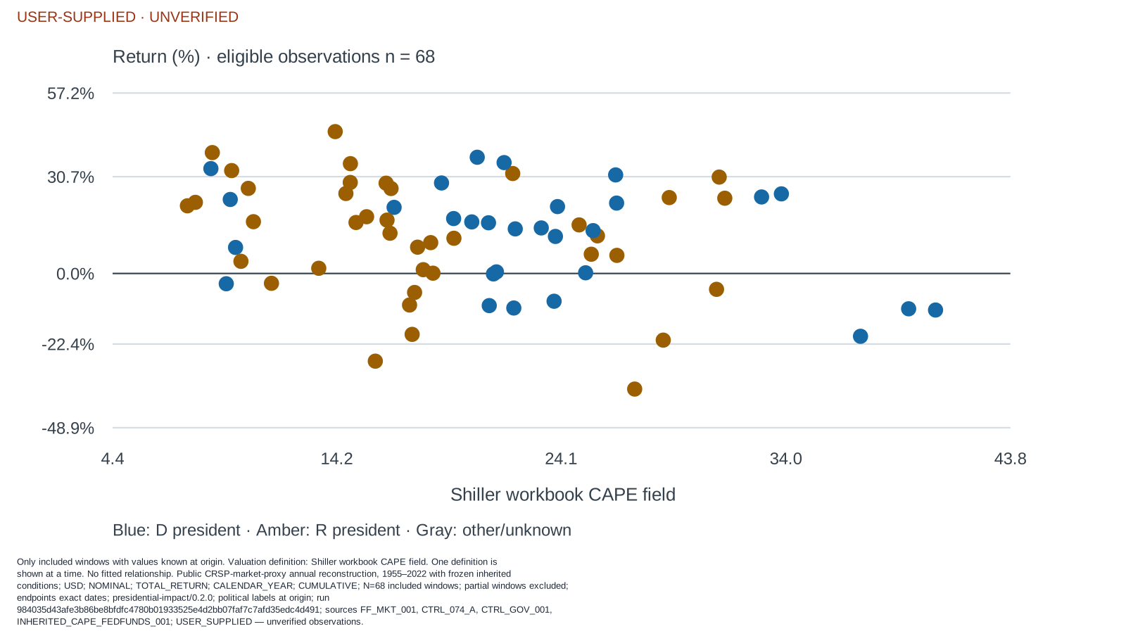
Figure 5. QuantMeridian PRES inherited-valuation view. Each dot is one eligible 1955–2022 annual window, colored by the president’s party at the window origin. No fitted line is shown: the intended claim is the descriptive pattern in the observed sample, not a predictive model with an implied slope.

The starting policy-rate level did not produce the same clean story. In the CRSP-market-proxy reconstruction, the lowest and highest policy-rate quartiles averaged 13.69% and 13.74%, respectively, and the pattern was non-monotonic in both constructions. A policy rate can matter immensely for discount rates, borrowing costs, and sector outcomes without its level alone providing a stable directional annual-equity-return rule.

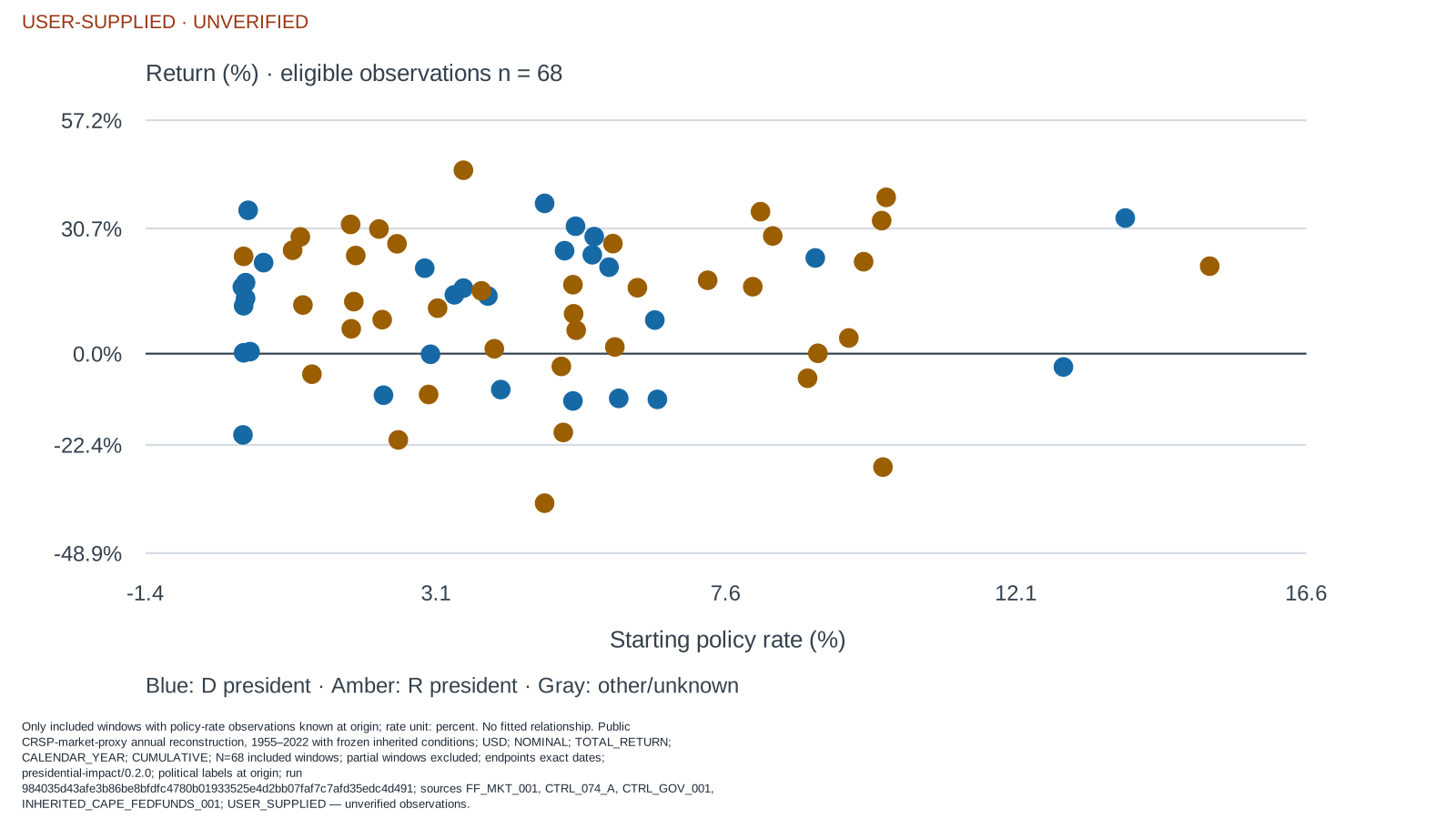
Figure 6. The matching policy-rate view. The wide vertical dispersion at both low and high starting rates makes the visual point more directly than a single correlation: the frozen sample does not provide a stable directional relationship from the level of the policy rate to the next annual equity return.

This is the distinction I would carry into an investment meeting:

Politics can change the mechanism. Starting conditions can change the odds.

Neither sentence is a portfolio rule. Together, they are a much better research agenda than asking which party has the prettier average.

What I would do with this as an investor

I would treat an election or a change in congressional control as a prompt for structured scenario work:

1. Identify the policy channels that could plausibly affect the portfolio: taxes, regulation, trade, fiscal spending, energy, health care, defense, labor, and capital costs.
2. Ask what the market already expects. A policy change that is widely priced may produce less return impact than a smaller surprise that was not.
3. Check valuation, earnings expectations, balance-sheet sensitivity, and exposure by sector or company before extrapolating from a national political average.
4. Define the risks that would falsify the scenario instead of letting a favorable election narrative silently become a position-sizing model.

This approach is less satisfying than a party-based market forecast. It is also closer to how investment decisions actually work. Equity returns are the joint output of starting valuation, growth, inflation, liquidity, risk appetite, global events, innovation, and policy. A political label is part of the map; it is not the terrain.

What this research does not establish

This project is deliberately unable to establish several tempting conclusions:

• It is not an exact replication of Fiduciary Trust International’s vendor- sourced S&P 500 analysis.
• It does not identify a causal effect of a president, party, or Congress on equity returns.
• It does not establish durable alpha, a four-year trading calendar, or a forecast for the next administration.
• It does not treat 87 annual rows—or 13 administrations in the inherited-conditions extension—as independent trials from a laboratory.

That is not a weakness to hide in a footnote. It is the reason the result is worth using carefully. A research process should tell you when a story is too small for the conclusion it is trying to carry.

The useful conclusion is not “ignore politics.” It is more demanding:

Use politics to ask better questions about mechanisms, valuation, and what is already priced. Do not confuse a historical average with a tradable signal.

Sources and method

• Fiduciary Trust International, “Should the balance of power in Washington matter to investors?” (October 16, 2024). Original research prompt; not reproduced exactly here.
• Kenneth R. French Data Library, U.S. Research Returns Data. Source of the public CRSP-market-proxy construction.
• Robert J. Shiller, online data. Source of the CAPE field and separately constructed S&P Composite robustness series.
• Federal Reserve, H.15 selected interest rates. Source family for the effective federal funds-rate input.
• National Archives, Twentieth Amendment term-date record. Authority for the January 20 presidential-term convention used in the cycle sensitivity.

All results use the project’s frozen local captures and reviewed political control inputs. The return sample ends in 2022 because the captured Shiller workbook does not provide the complete trailing-dividend data required to build the 2023 robustness return without imputation. This is research context, not investment advice.